Find Percentages Duplicate the table and create a percentage of total item for each using the formula below (Note: use $ to lock the column reference before copying + pasting the formula across the table). Each total percentage per item should equal 100%. Add Data Labels on Graph Click on Graph Select the + Sign Check Data Labels To display percentage instead of the general numerical value, Create one secondary data table and convert all the general numerical values into percentages. Then click one of the data labels of the stacked column chart, go to the formula bar, type equal (=), and then click on the cell of its percentage equivalent.

Trick to solve percentage. Percentage study material covers tricks of percentage, shortcuts of
Select the data range that you want to create a chart but exclude the percentage column, and then click Insert Column or Bar Chart2-D Clustered Column Chart . After inserting the chart, then, you should insert two helper columns, in the first helper column-Column D, please enter this formula: =B2*1.15 =B2&CHAR (10)&" ("&TEXT (C2,"0%")&")" 📊 Master Excel Charts: Display Percentage % and Value in Column Charts! 📈🔥 Unlock the power of Excel charts with this step-by-step tutorial! Learn how to. 1. Make a Percentage Vertical Bar Graph in Excel Using Clustered Column For the first method, we're going to use the Clustered Column to make a Percentage Bar Graph. Steps: Firstly, select the cell range C4:D10. Secondly, from the Insert tab >>> Insert Column or Bar Chart >>> select Clustered Column. This will bring Clustered Vertical Bar Graph. The Column Chart with Percentage Change. This post was inspired by a chart I saw in an article on Visual Capitalist about music industry sales. If you want to display both the counts and the percentage value, you need to pass in the counts and use the Chart Designer to calculate the percentages from the counts. Reply. Karlos says: January 30.

Percentage Sign Free Stock Photo Public Domain Pictures
1 Building a Stacked Chart. 2 Labeling the Stacked Column Chart. 3 Fixing the Total Data Labels. 4 Adding Percentages to the Stacked Column Chart. 5 Adding Percentages Manually. 6 Adding Percentages Automatically with an Add-In. 7 Download the Stacked Chart Percentages Example File. Click "Calculate." The calculator will show that your food expenses account for 25% of your monthly budget. FAQs? Q1: What types of charts can benefit from the Chart Percentage Calculator? Occasionally you may want to show percentage labels in a stacked column chart in Excel. This tutorial provides a step-by-step example of how to create the following stacked bar chart with percentage labels inside each bar: Let's jump in! Step 1: Enter the Data Step 3: Apply the percentage to the data label of your Excel chart. Now, In the option's label (the icon that looks like a chart), you see the Percentage option. Click on this option to instantly convert your data label into the percentage of the total in your Excel chart Step 4: Display multiple values in the labels
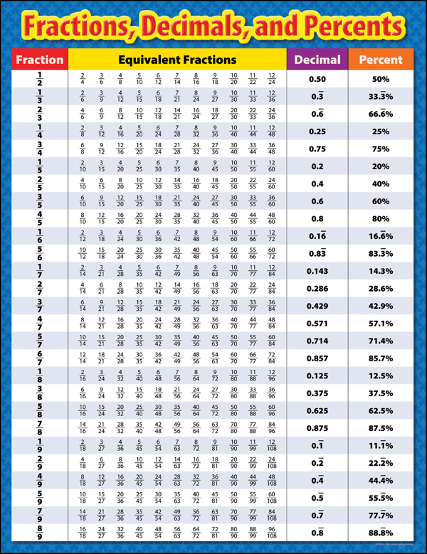
Fractions, Decimals, and Percents Chart Creative Teaching Press 9781606894101
Pie chart with percentage is ready. The chart shows the percentage of income from taxation. 100% Stacked Column. Let's add columns to the table: with a percent (the percentage contribution of each type of tax in the total amount); 100%. We click on any cell of the table. Go to the tab "INSERT". In the group of "Carts" choose "100% Stacked. Adding percentages to Excel charts provides valuable context and insight for the audience Review and format the data properly before creating the chart Select the appropriate chart type and add data labels to the chart Format the data labels to display percentages and ensure readability
Then click the Table icon under the Visualizations tab. Then drag Store to the Columns panel and drag Sales to the Columns panel twice: Next, right click on the first Sum of Sales and then hover over Conditional formatting, then click Data bars: Next, right click on the second Sum of Sales and then hover over Show value as, then click Percent. To create a percentage chart in Google Sheets, you first need to select the data that you want to include in the chart. This data should include the values or numbers that will be used to calculate the percentages. Once you have selected the data, you can proceed to the next step of creating the percentage chart.

How to create a chart with both percentage and value in Excel?
In this method, we will use the basic line graph feature to make a percentage line graph in Excel. We will utilize the following dataset for this purpose. 📌 Steps: First, select Range B5:C9. Then, go to the Insert tab. After that, choose the Line with Markers option from the chart list. Now, look at the following graph. What is Percentage Math? In mathematical form, the percentage of a given quantity can be defined as: "A comparative value that indicates the hundredth part of a quantity" In simple words, we can say that percentage is a number or ratio can be represented in the form of a fraction as per hundreds (100) of that number.
