The AD-AS (aggregate demand-aggregate supply) model is a way of illustrating national income determination and changes in the price level. We can use this to illustrate phases of the business cycle and how different events can lead to changes in two of our key macroeconomic indicators: real GDP and inflation. Key Features of the AD-AS model 5 May 2017 by Tejvan Pettinger Diagrams showing how shifts in aggregate demand (AD) and aggregate supply (AS) affect macroeconomic equilibrium - real GDP and price level (PL) Includes short-run aggregate supply (SRAS) and long-run aggregate supply (LRAS) and classical and Keynesian view of LRAS curves.
Unit 3 Aggregate Demand Supply and Fiscal Policy
The AD-AS or aggregate demand-aggregate supply model (also known as the aggregate supply-aggregate demand or AS-AD model) is a widely used macroeconomic model that explains short-run and long-run economic changes through the relationship of aggregate demand (AD) and aggregate supply (AS) in a diagram. In an AD/AS diagram, long-run economic growth due to productivity increases over time is represented by a gradual rightward shift of aggregate supply. The vertical line representing potential GDP—the full-employment level of gross domestic product—gradually shifts to the right over time as well. Lesson summary: equilibrium in the AD-AS model In this lesson summary review and remind yourself of the key terms and graphs related to a short-run macroeconomic equilibrium. Topics include how to model a short-run macroeconomic equilibrium graphically as well as the relationship between short-run and long-run equilibrium and the business cycle. We can use the AD-AS model to help explain the business cycle (in other words, the recessions and booms that we have seen in the real world). When AD or SRAS curves shift, we call these "shocks". Why a shock? Because the change come as a complete surprise!
Solved Use the AD/AS model to graph and explain what happens
Equilibrium in the AD-AS Model Aggregate demand and aggregate supply curves Google Classroom The concepts of supply and demand can be applied to the economy as a whole. Key points Aggregate supply is the total quantity of output firms will produce and sell—in other words, the real GDP. What is the equilibrium? Step 1. Draw your x- and y-axis. Label the x-axis "Real GDP" and the y-axis "Price Level." Step 2. Plot AD on your graph. Step 3. Plot AS on your graph. Step 4. Look at Figure 2, which provides a visual to aid in your analysis. Figure 2. The AS-AD Curves AD and AS curves created from the data in Table 1. Step 5. Plot AS on your graph. Step 4. Look at Figure 2, which provides a visual to aid in your analysis. Figure 2. The AS-AD Curves AD and AS curves created from the data in Table 1. Step 5. Determine where AD and AS intersect. This is the equilibrium with the price level at 130 and real GDP at $680. Step 6. The aggregate demand/aggregate supply, or AD/AS, model can be used to illustrate both Say's Law and Keynes' Law. Say's Law states that supply creates its own demand; Keynes' Law states that demand creates its own supply. Take a look at the AD/AS diagram below.
AS/AD
In the AD-AS diagram, cyclical unemployment is shown by how close the economy is to the potential or full employment level of GDP. Returning to Figure 1 above, cyclical unemployment increases when the output falls substantially below potential GDP on the AD-AS diagram, as at the equilibrium point E 0. Figure 2. The aggregate demand curve, or AD curve, shifts to the right as the components of aggregate demand—consumption spending, investment spending, government spending, and spending on exports minus imports—rise. The AD curve will shift back to the left as these components fall.
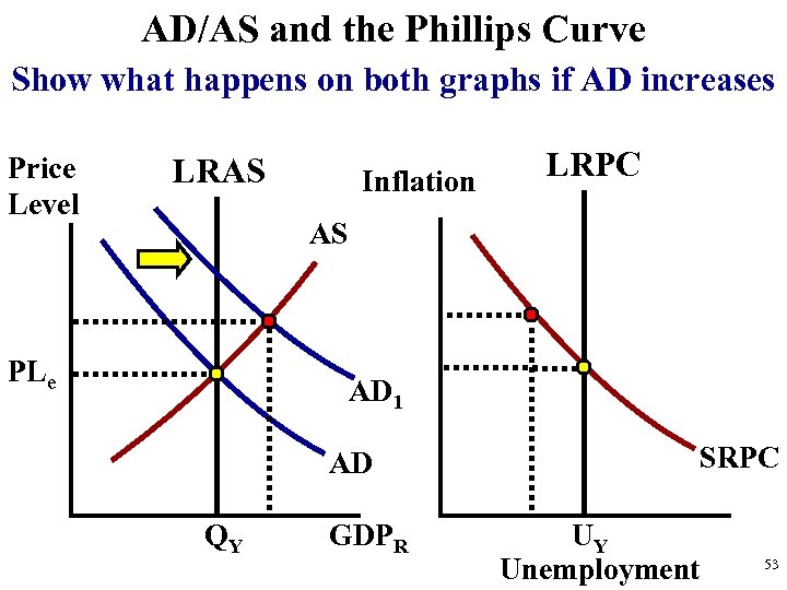
AD-AS Model Graph. Figure 1 illustrates the AD-AS model. In this graph, notice three important curves: Aggregate demand (AD), Short-run aggregate supply (SRAS), and long-run aggregate supply (LRAS). Fig. 1 - AD-AS model graph. Aggregate demand refers to the total demand for goods and services within the economy. AP Macroeconomics Study Guide. VII. AD/AS Graph. Aggregate Demand Shifters. These cause shifts in aggregate demand: C C (consumer wealth, consumer expectations, household indebtedness, taxes) I I (interest rates, expected returns on investment, business taxes, technology, degree of excess capacity) G G. Xn X n (National income abroad, exchange.

1303AFE Sem 2 ADAS Graph Example YouTube
The AD/AS diagram shows cyclical unemployment by how close the economy is to the potential or full GDP employment level. Returning to Figure 24.9, relatively low cyclical unemployment for an economy occurs when the level of output is close to potential GDP, as in the equilibrium point E 1. The AD curve slopes down, which means that increases in the price level of outputs lead to a lower quantity of total spending. The reasons behind this shape are related to how changes in the price level affect the different components of aggregate demand.. Plot AD on your graph. Step 3. Plot AS on your graph. Step 4. Look at Figure 24.5.
