Often you may want to create a summary table in Excel to summarize the values in some dataset. Fortunately this is easy to do using built-in functions in Excel. The following step-by-step example shows how to create a summary table in Excel in practice. Step 1: Enter the Original Data 1. Using UNIQUE and SUMIFS Functions to Create Summary Table in Excel Microsoft 365 has quite amazing features like the UNIQUE function. So in this process, we are going to use UNIQUE and SUMIFS functions. 📌 Steps: In the first step, we just use the UNIQUE function and select the whole Continent column.

Excel Summary Table Hot Sex Picture
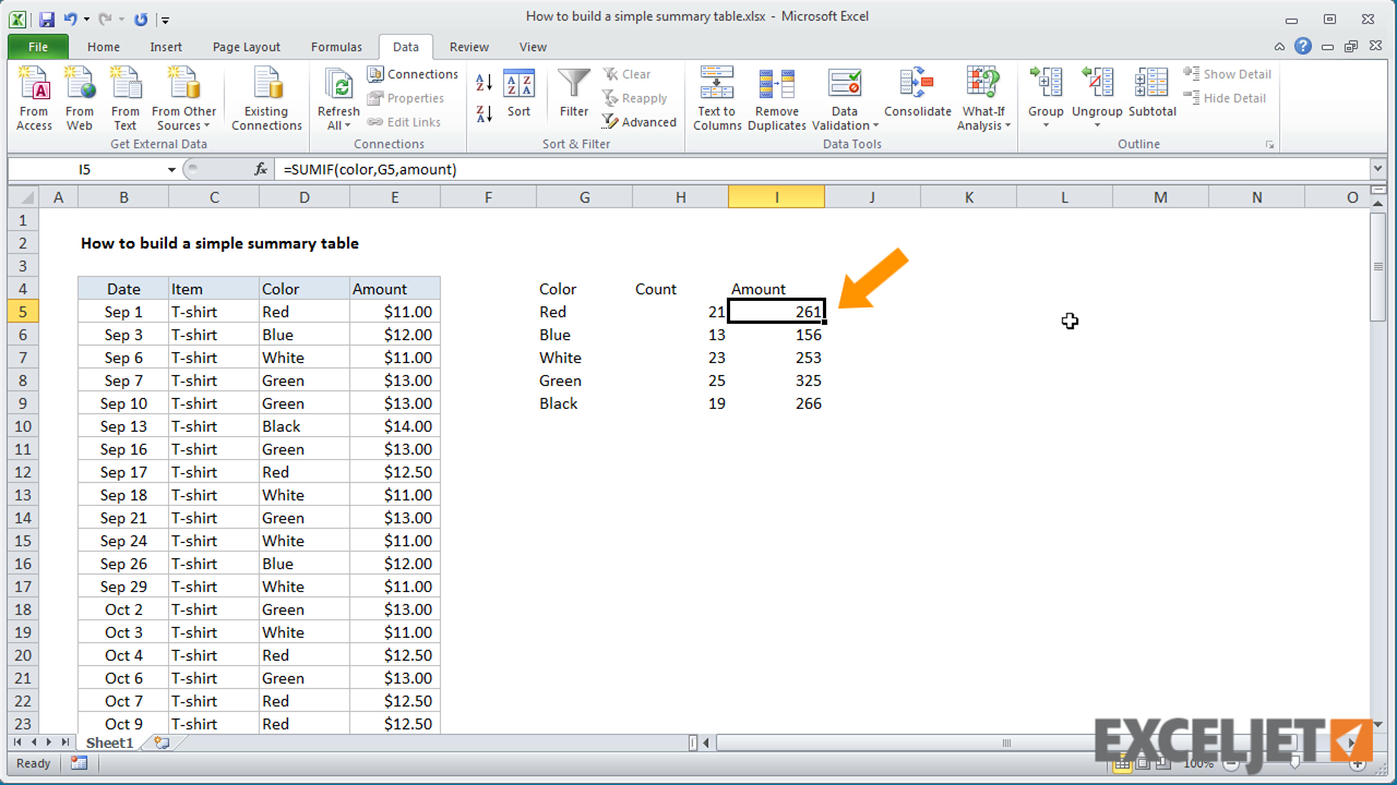
Summary tables in Excel are essential for organizing and analyzing data effectively. Understanding the data and identifying key data points is crucial for creating a useful summary table. Properly organizing and formatting the data in Excel is important for preparing to create a summary table. Download Workbook A summary table should include a unique list of categories. Creating a unique list of categories can become tedious as you keep adding more items in the future. To keep things simple and automate this task, you essentially can use either one of the two methods: Pivot Table or Excel formulas. Let's take a look at both. Pivot Tables are fantastic tools for summarizing data, but you can also use formulas to build your own summaries using functions like COUNTIF and SUMIF. See how in this 3 minute video. Transcript In this video, I want to show you how to build a quick summary table using the COUNTIF and SUMIF functions. Summarize Data With an Excel Table Using Slicers to Summarize by different dimensions Summarize With Excel Pivot Tables Summarize Data With Excel Functions Advanced Excel Functions for Summarizing Data Summarize With Descriptive Statistics From Analysis Toolpak You can apply the different ways to summarize data based on your familiarity with Excel.

How to Create a Summary Table in Excel (With Example) Statology
Step 1: Select your data To create a Pivot Table, start by selecting the data range that you want to summarize. This can include multiple columns and rows of data. Step 2: Navigate to the "Insert" tab Once you have selected your data, navigate to the "Insert" tab in Excel and click on the "Pivot Table" option. A summary table allows you to consolidate and display key information in a clear and easily digestible format, making it easier to analyze and draw insights from your data. Here's how you can set up a summary table in Excel. A. Identifying the data to be included A summary table in Excel can significantly simplify the data analysis process. It allows for the summarization and consolidation of large datasets into a more manageable format. Creating a summary table is an essential skill for business analysts, students, and researchers. Summary tables in Excel are essential for summarizing and analyzing data in a quick and organized manner. Using summary tables can save time and effort in the data analysis process, and present findings in a professional manner. Organizing data in a tabular format and removing blank rows or columns is important for setting up a summary table.
Excel Tables How To Excel
1. To display rows for a level, click the appropriate outline symbols. 2. Level 1 contains the total sales for all detail rows. 3. Level 2 contains total sales for each month in each region. 4. Level 3 contains detail rows — in this case, rows 17 through 20. 5. The most effective way to create a summary table in Excel from multiple worksheets is to use the Power Query Editor and PivotTable. Let's go through the procedure below for a detailed description. Steps: We will be using the following sheets to create the summary table from multiple worksheets.
A PivotTable is a powerful tool to calculate, summarize, and analyze data that lets you see comparisons, patterns, and trends in your data. PivotTables work a little bit differently depending on what platform you are using to run Excel. Windows Web Mac iPad Create a PivotTable in Excel for Windows PivotTables from other sources 1. Apply AutoSum Option to Summarize Data Now we want to summarize the data given below. Let's first calculate the total amount of sales. We can do that by using AutoSum functions. Follow the steps below. Steps: Click on the cell where you want to display the sum. Here we have selected H4.
Excel Summary Table shiftlasopa
Steps: First, open a new worksheet and create a dataset ( B4:C7) like the screenshot below. Secondly, select the cell next to the cell of Total Marks of Math. Thirdly, go to the Home tab. Then, go to the Editing group and click on the AutoSum option. As a result, the SUM function will automatically appear in the cell just like the screenshot below. This chapter's file already has the main table separated into two Biannual worksheets with an appropriate Excel basic table on each, then a Pivots worksheet in which Pivot tables have already been created from those two Biannual Excel basic tables. In Ch19-Summary.xlsx, go into the Pivots worksheet. The Pivot tables are currently sorted by.
